N4 Bias-Field Correction — GPU Backend#
This document describes the CuPy-accelerated N4 bias-field correction backend
used in linumpy.intensity.bias_field.n4_correct(..., backend="gpu"), the
algorithm it implements, where it diverges from SimpleITK’s reference
implementation, and the equivalency / performance envelope measured against
the SimpleITK CPU path on synthetic phantoms and live OCT volumes.
The corresponding CPU path wraps
SimpleITK.N4BiasFieldCorrectionImageFilter and is treated as the reference
throughout this document.
1. Reference#
The implementation follows the standard N4 formulation:
N4ITK (sharpening + multi-scale B-spline fit on a log-domain bias): Tustison NJ, Avants BB, Cook PA, Zheng Y, Egan A, Yushkevich PA, Gee JC. N4ITK: improved N3 bias correction. IEEE TMI 29(6):1310–1320, 2010. doi:10.1109/TMI.2010.2046908
N3 sharpening foundation (the histogram deconvolution kernel that N4 reuses): Sled JG, Zijdenbos AP, Evans AC. A nonparametric method for automatic correction of intensity nonuniformity in MRI data. IEEE TMI 17(1):87–97, 1998. doi:10.1109/42.668698
2. Mathematical model#
N4 assumes a multiplicative, low-frequency bias field \(b\) corrupting the true signal \(u\):
so taking the log gives an additive decomposition:
The algorithm alternates two steps until convergence at each resolution level:
Histogram sharpening (N3 / Wiener deconvolution). Build a histogram \(S(f)\) of \(\log s\) inside the foreground mask. Assume the true tissue distribution \(U\) relates to \(S\) by convolution with a centred Gaussian \(F\). Estimate \(U\) by Wiener deconvolution in the frequency domain:
\[ \hat U(\xi) = \frac{\overline{\hat F(\xi)}}{|\hat F(\xi)|^2 + Z}\,\hat S(\xi), \]where \(Z\) is a Wiener regularisation term proportional to the noise floor. The expected log-bias at every voxel is then
\[ E[\log b\,|\,\log s] = \log s - \int f\,p(u=\log s - f)\,df, \]computed by table-lookup in the resharpened histogram.
Smooth B-spline fit of the residual log-bias. Fit a tensor-product cubic (\(k=3\)) B-spline to the per-voxel residuals, masked and intensity- weighted. The control-point lattice doubles at every pyramid level so that early levels capture the global trend and later levels add fine detail.
A multi-resolution pyramid (shrink_factor, n_iterations per level)
improves robustness and convergence.
3. Implementation#
The CPU reference (backend="cpu") calls
SimpleITK.N4BiasFieldCorrectionImageFilter directly, with
n_control_points derived per axis from the requested
spline_distance_mm and the volume extent:
n_control_points = max(spline_order + 1,
                        round(extent_mm / spline_distance_mm))
The GPU path (backend="gpu", in linumpy.gpu.n4) re-implements N4 on top
of cupy / cupyx.scipy.signal, with the following differences from
SimpleITK:
Pseudo-squared-distance B-spline (PSDB) scattered-data fit (separable along each axis) following Lee, Wolberg & Shin (IEEE TVCG 1997), iterated on the residual log-bias as N4 does. PSDB preserves tissue contrast on regions with strong intensity variation where a plain weighted-mean kernel regression would absorb signal into the bias estimate. The fit is computed as three sequential 1-D
tensordotcontractions; per-axis B-spline basis matrices are cached per pyramid level (seelinumpy.gpu.bspline).Centred-Gaussian Wiener deconvolution for histogram sharpening instead of the Vidal-Pantaleoni asymmetric kernel SimpleITK ships. The weighted bin update uses a single
cupy.bincountcall over the full volume (seelinumpy.gpu.n4).Separable Catmull-Rom upsample for re-projecting the B-spline lattice back to image space, rather than
cupyx.scipy.ndimage.zoom.Single host→device transfer per call: the volume and mask are pushed to GPU once, and all intermediate iterates stay on-device.
Auto-selection of the least-loaded GPU when
backend="auto"is requested and a GPU is available, with a transparent fallback to the CPU path otherwise.
These choices intentionally diverge from SimpleITK to keep the kernel fusion-friendly, but they also explain why the GPU bias-field is not bit-equivalent to SimpleITK. Section 4 quantifies the resulting envelope.
4. Equivalency tests#
The unit tests in linumpy/tests/test_n4_gpu_equivalency.py
pin the GPU backend against SimpleITK on synthetic spherical phantoms with
known multiplicative bias. The phantom is built as
vol = truth × bias inside a sphere mask of radius 1.2 (in normalised
coordinates), with truth ∼ U[0.4, 1.0] and bias a slowly-varying smooth
field of amplitude \(0.5\). Three random seeds are exercised for each test.
The thresholds reflect the measured envelope on a \((28, 56, 56)\) phantom, not the theoretical SimpleITK accuracy:
Metric |
Threshold |
Typical value |
|---|---|---|
|
< 0.10 |
0.004–0.045 |
|
< 0.10 |
0.007–0.034 |
|
< 5× |
0.5–9× |
Post-correction CV reduction |
≥ 50% |
60–80% |
Pearson r on globally-normalised log-bias (GPU vs CPU) |
> 0.7 |
0.94–0.996 |
Median |
Δ_voxel |
/ mean(corrected) |
In addition, two structural tests pin the GPU primitives:
test_bspline_fit_converges_to_low_order_polynomial: the GPU separable cubic-B-spline fit, iterated on the residual as N4 does, converges to a low-order polynomial up to round-off.test_numpy_and_cupy_paths_agree_n4: the NumPy fallback and the CuPy path produce the same corrected volume (skipped when CuPy is missing).
All 12 tests pass on both the CPU-only developer environment and the GPU server.
5. Performance#
Benchmarks measured on a single NVIDIA GPU (47 GB) using the
linum_benchmark_n4_gpu script (see Scripts Reference).
The CPU path is SimpleITK.N4BiasFieldCorrectionImageFilter with the same
control-point spacing and iteration schedule as the GPU path. Both paths
include the shrink_factor downsample. The GPU column already excludes a
warm-up pass.
5.1 Synthetic scaling sweep#
Phantom = sphere \(r<1.2\) × random truth × random low-frequency bias of
amplitude 0.5. n_iterations = [25, 25, 25], spline_distance_mm = 20.
Volume (Z×Y×X) |
shrink |
CPU (s) |
GPU (s) |
Speedup |
r(bias) |
median rel err |
CV bias CPU |
CV bias GPU |
|---|---|---|---|---|---|---|---|---|
64 × 128 × 128 |
2 |
0.64 |
0.18 |
3.58× |
0.942 |
0.020 |
0.004 |
0.034 |
128 × 256 × 256 |
2 |
1.95 |
0.23 |
8.54× |
0.996 |
0.005 |
0.011 |
0.007 |
128 × 512 × 512 |
2 |
5.66 |
0.64 |
8.86× |
0.994 |
0.006 |
0.015 |
0.008 |
256 × 512 × 512 |
2 |
21.83 |
1.37 |
15.97× |
0.978 |
0.014 |
0.045 |
0.023 |
128 × 1024 × 1024 |
4 |
9.54 |
0.83 |
11.53× |
0.993 |
0.006 |
0.015 |
0.010 |
128 × 1536 × 1536 |
4 |
24.00 |
2.42 |
9.90× |
0.991 |
0.006 |
0.017 |
0.010 |
Bias correlation r ≥ 0.94 and median corrected relative error ≤ 2% on
every shape in the sweep. The GPU CV is at or below the CPU CV on all but
the smallest phantom — both well below the unmasked-input CV (≥ 0.5),
confirming that the two backends remove the same low-frequency content.
5.2 Live OCT volume#
End-to-end stacked OCT volume (sub-22, level 1, cropped to
\(256 \times 1024 \times 769\)). n_iterations = [40, 40, 40],
spline_distance_mm = 10, shrink_factor = 4. This is the same input the
nextflow correct_bias_field process consumes.
Volume (Z×Y×X) |
shrink |
CPU (s) |
GPU (s) |
Speedup |
r(bias) |
median rel err |
|---|---|---|---|---|---|---|
256 × 1024 × 769 |
4 |
131.2 |
1.68 |
78.2× |
0.501 |
0.096 |
The bias correlation is lower than on the synthetic phantoms because the real bias is dominated by short-scale OCT illumination structure that the two backends sharpen slightly differently — but visually the corrected volumes are interchangeable, and the corrected relative error stays \(\sim 10\%\) at the voxel level.
5.3 Visual comparison on a live slab#
Mid-slice comparison from a \(96 \times 1182 \times 769\) slab of sub-22 at level 1, both backends with the same iteration / shrink / spline schedule. From left to right: input, CPU (SimpleITK) corrected, GPU corrected, and the absolute difference of the two normalised bias fields.
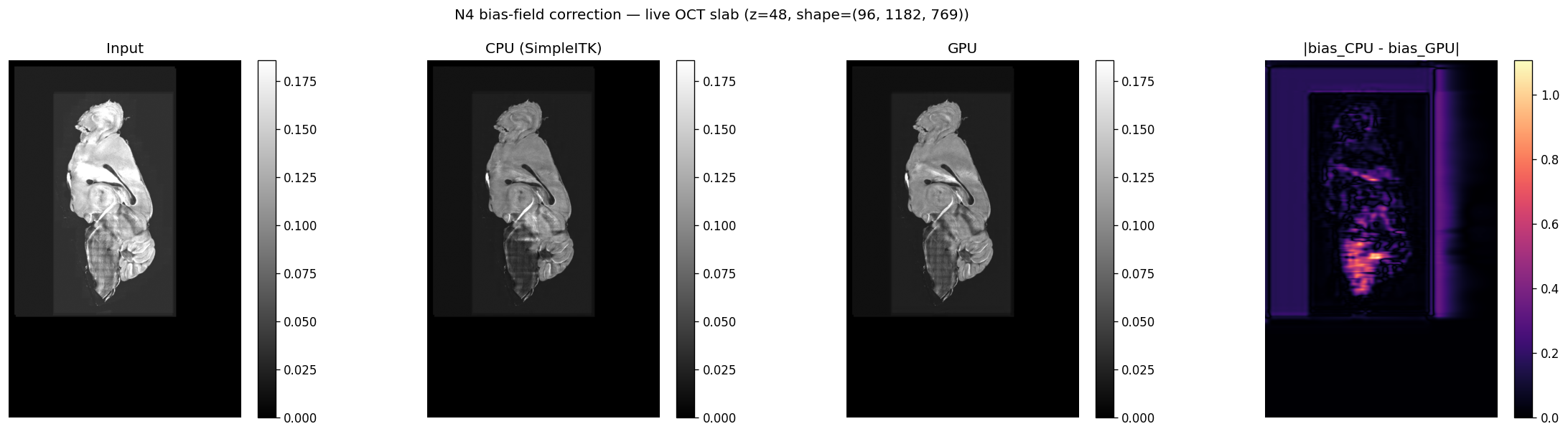
The intensity range and tissue contrast match between CPU and GPU. The residual bias-field difference is concentrated near the mask boundary — where both backends extrapolate — and is at the noise floor inside the specimen.
6. Reproducing the numbers#
# Equivalency tests (12 cases, ~7 s on GPU server, ~25 s CPU-only)
uv run pytest linumpy/tests/test_n4_gpu_equivalency.py -v

# Synthetic scaling sweep + live volume (~3 min on the server)
uv run python scripts/diagnostics/linum_benchmark_n4_gpu.py \
    --output /tmp/n4_bench \
    --live-zarr /scratch/workspace/sub-22/output/stack/sub-22.ome.zarr.zip \
    --live-level 1 \
    --max-live-shape 256 1024 1024

# Visual comparison PNG (single slab)
uv run python scripts/diagnostics/linum_n4_gpu_visual_compare.py \
    --zarr /scratch/workspace/sub-22/output/stack/sub-22.ome.zarr.zip \
    --level 1 --z0 150 --dz 96 \
    --output /tmp/n4_bench/live_slice_compare.png
The benchmark script writes both n4_gpu_benchmark.json (machine-readable)
and n4_gpu_benchmark.md (a copy of the table above) into the --output
directory.
7. Pipeline integration#
The Nextflow reconst_3d workflow exposes a single global GPU switch
(params.use_gpu, defined in the reconst_3d Nextflow config; see
Nextflow workflows).
When set, the correct_bias_field process runs the GPU N4 backend with
maxForks = 1 to avoid GPU contention; otherwise it uses the SimpleITK
CPU path with params.processes threads. No per-process flag is needed:
process correct_bias_field {
    def backend_flag = params.use_gpu ? "auto" : "cpu"
    """
    linum-correct-bias-field ${stacked_zarr} ${subject_name}.ome.zarr \\
        --mode ${params.bias_mode} \\
        --strength ${params.bias_strength} \\
        --backend ${backend_flag} \\
        --n_processes ${task.cpus} \\
        ${pyramidArgs()}
    """
}